
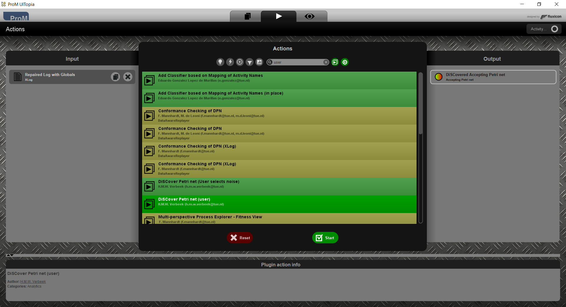
Today, version 6.13.62 of the DiSCover package has been released. This release introduces a wizard that guides you through the configuration of the DiSCover algorithm. The wizard consists of 8 steps, which are introduced next. As working example we use the example event log from the following paper:
Advanced Process Discovery Techniques. In: Aalst, W. M. P.; Carmona, J. (Ed.): Process Mining Handbook, vol. 448, pp. 76–107, Springer, Cham, 2022.
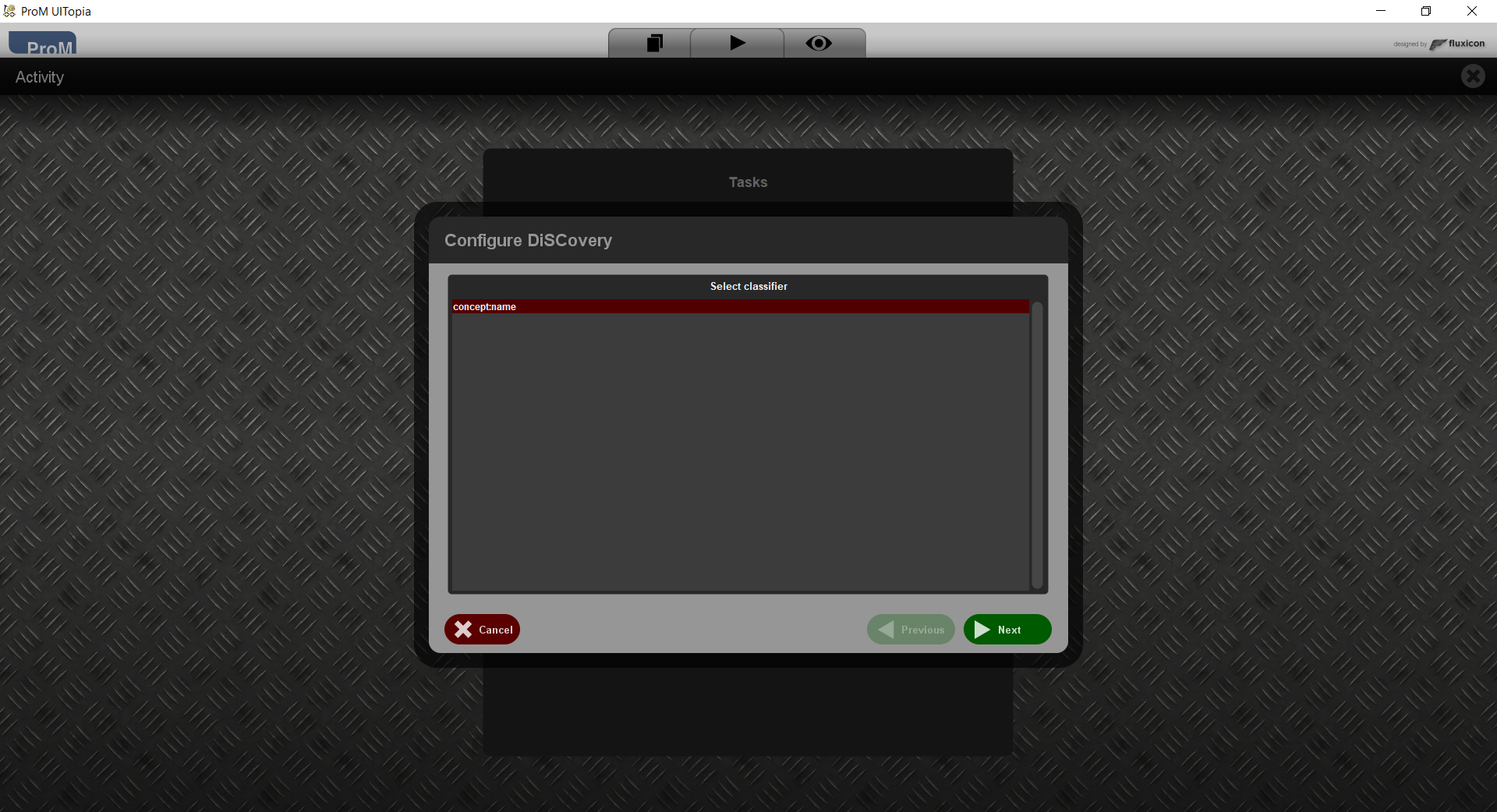
This step shows all classifiers from the log, or the concept:name classifier if the log has no classifiers.
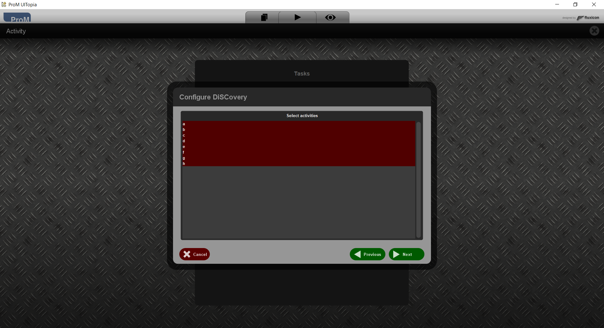
Only selected activities will be taken into account in the remainder.
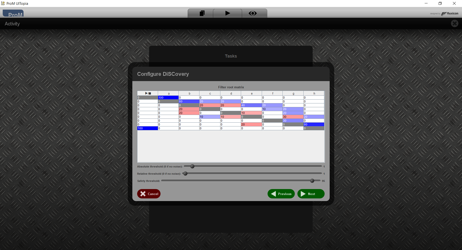
This step shows the root directly-follows matrix, that is, the directly follows matrix for the event log and the selected events. A red cell indicates that the row activity can directly follow the column activity and vice versa, that is, these activities may be concurrent. A blue cell indicates that the row activity can be directly followed by the column activity, but not vice versa.
The matrix can be filtered using the sliders below, or by directly editing the cells. A positive number indicates a directly-follows relation, an negative number indicates no directly follows relation, and 0 indicates indifference. If you as a user know that b and c are not concurrent, you can set the value 0 for either the cell (b,c) or the cell (c,b).
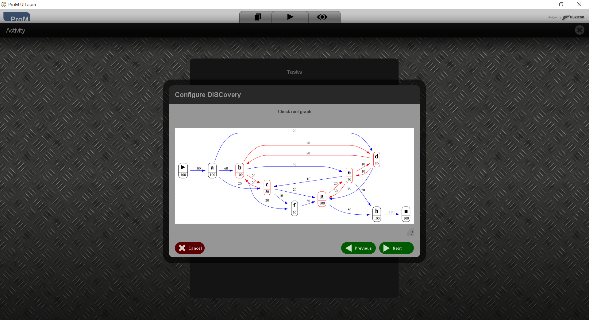
This shows the directly-follows graph that will be used to split the event logs into components. Basically, a single component is obtained by removing activities such that concurrency (red arrows) is removed. As an example if we remove b and e from the picture, then no red arrows remain.
Here you can check whether you agree with this graph. If not, you can go back to the earlier step to filter the matrix further.
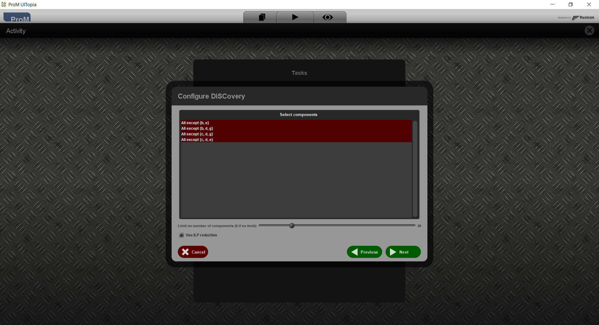
This shows all components that were found. As an example the top component is the component with b and e removed.
Below, you can configure whether you want to automatically reduce the number of components (useful if there are many) and whether you want to use an ILP for this. Using an ILP may result in a more sensible subset of components, but it may take much time.
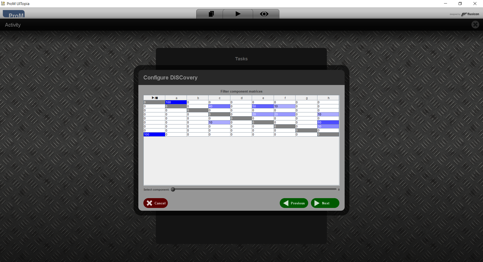
This shows the matrix that was constructed for every component. Using the slider below, you can move from one matrix to the next and back.
You can filter any component matrix by directly editing a cell. This way, you can prevent an edge from being included, or you can enforce an edge to be included. As an example, if you are sure that a should never directly be followed by c, then you can change the value 40 in the corresponding cell to 0.
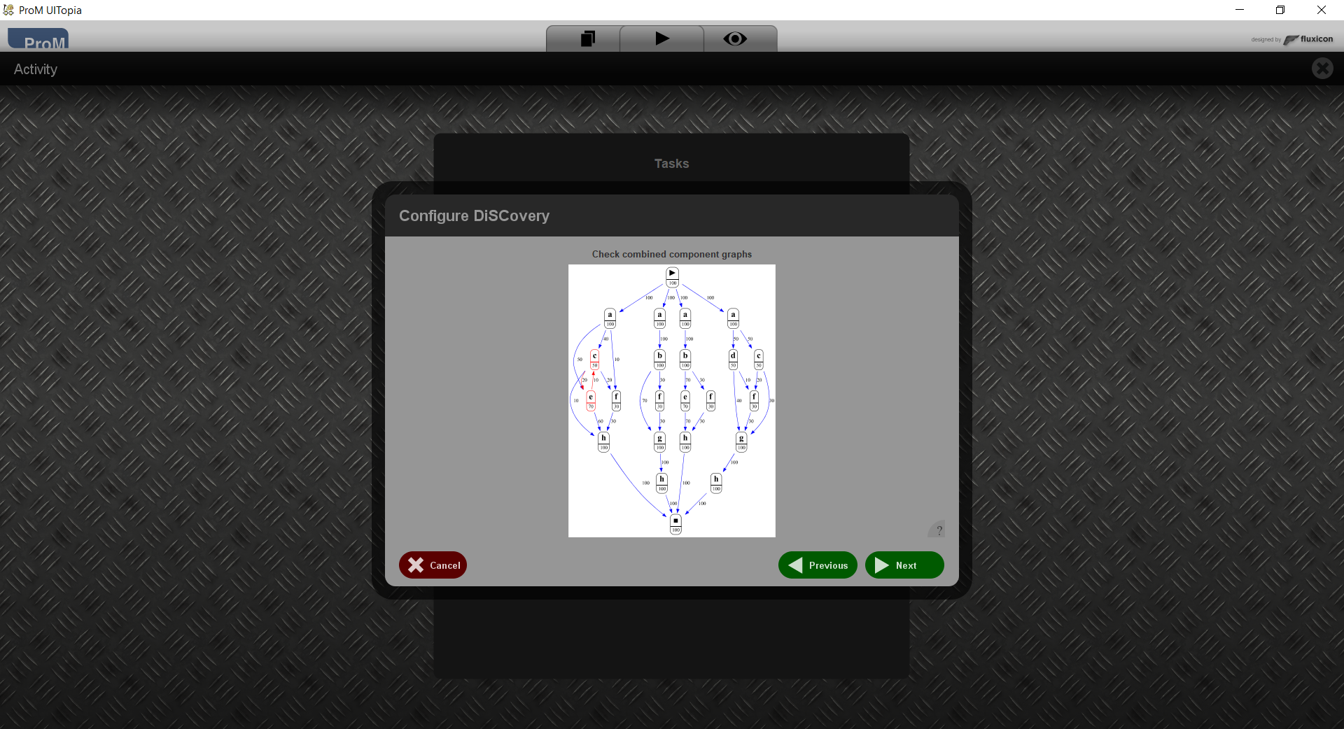
This shows the component graphs combined in a single graph. If you are not happy with these graph, you can go back to an earlier step and make changes. As an example if you do not like the short loop in the left-most graph between c and e, then you could go back to Step 5 and deselect any component that does not exclude both c and e.
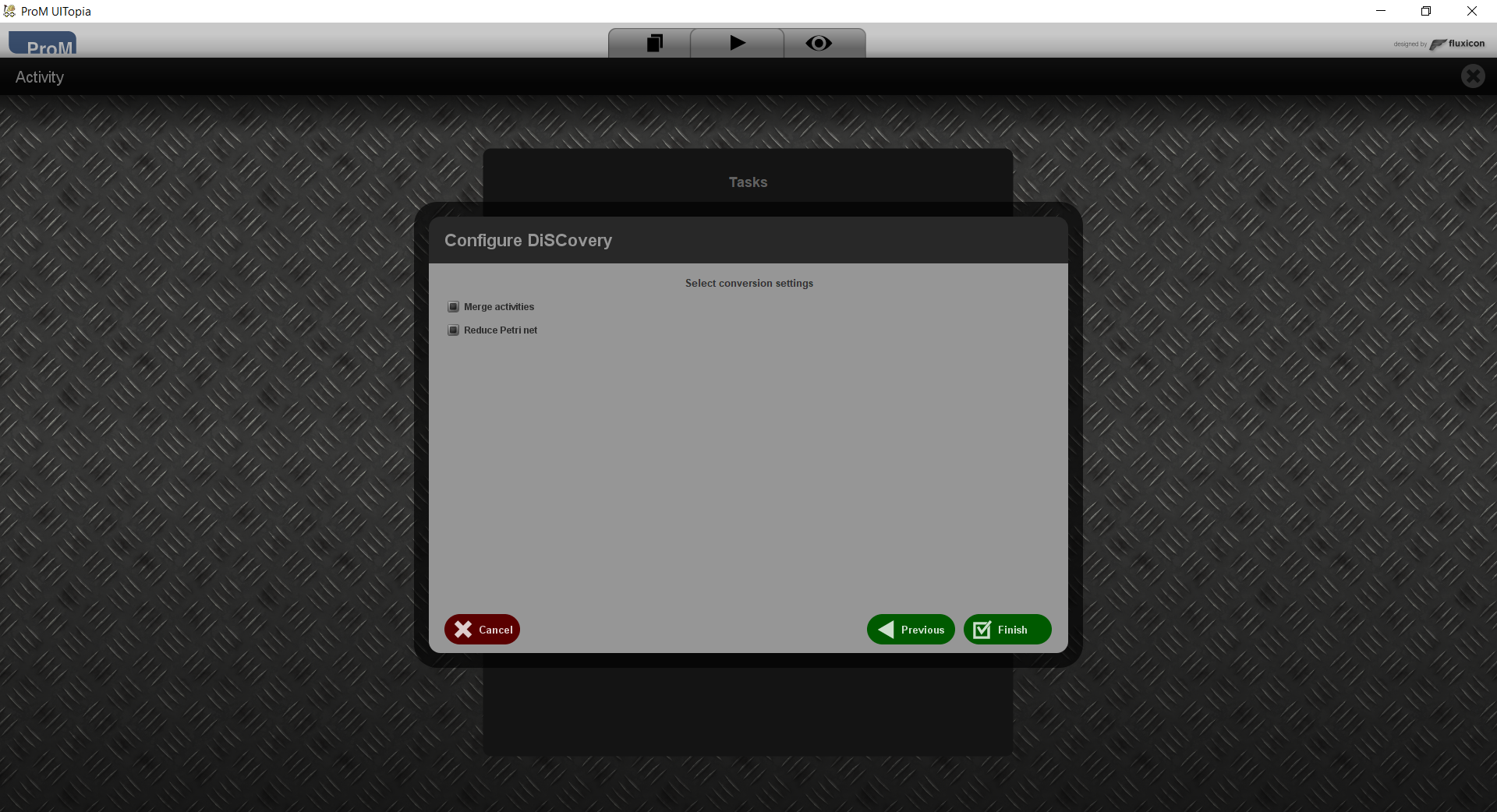
This step allows you to configure the way the graphs are converted into a Petri net.
